


Downtime costs businesses millions, but predictive maintenance can help you avoid them. Here’s how you can calculate the financial benefits of avoiding unplanned outages:
Key Takeaways:
- Calculate Baseline Costs: Start by measuring lost production, labor, scrap, and emergency repair expenses during downtime.
- Model Failure Risks: Use tools like probabilistic aging models to predict when assets might fail and schedule timely maintenance.
- Estimate Savings: Predictive maintenance reduces unplanned downtime by 30–45%, slashes emergency repair costs by 70–90%, and extends asset life by 20–40%.
- Prove ROI: Use metrics like downtime savings, maintenance cost reductions, and asset life extension to calculate ROI. Many programs achieve payback in 6–18 months with a 10:1 ROI.
By focusing on high-impact assets and using predictive tools, you can turn reactive maintenance into a cost-saving, efficiency-driven strategy.
Predictive Maintenance Secrets: ROI and Operational Efficiency – UpKeep
sbb-itb-5be7949
How to Calculate Baseline Downtime Costs
Determining baseline downtime costs is a key step in showing the financial advantages of predictive maintenance. Start by calculating the costs of unplanned downtime. This baseline acts as a benchmark for tracking improvements by considering both the lost hours and their financial consequences.
Measuring Total Outage Hours
To measure downtime effectively, analyze the past 12 months of data from your CMMS (or production logs). Apply a 1.8 multiplier to average repair times to account for secondary effects and unrecorded impacts. This approach captures not only full outages but also micro-stops and recovery periods when equipment operates below its peak efficiency [2][5][7]. Automated monitoring systems can help identify these smaller disruptions.
Recovery periods are particularly important to consider. During this time – typically 1–3 hours – equipment operates at reduced efficiency. Production rates drop, and scrap rates can rise by 20–40% [4][3]. Once you’ve gathered this data, translate the outage hours into financial terms.
Calculating the Financial Impact
After quantifying outage durations, the next step is to assess their financial impact. Use the following formula to calculate the Total Downtime Cost (TDC):
TDC = Lost Production Revenue + Labor Burden + Restart Costs + Quality/Scrap Costs + Emergency Maintenance Expenses + Contractual Penalties [7].
For lost production, focus on gross margin (revenue minus variable costs like materials and energy) instead of total revenue. This is especially important when determining downtime costs, as it provides a clearer picture of the financial impact. If the failed equipment is a production bottleneck, the hourly profit potential is lost entirely. However, if it’s not, operational buffers may absorb minor interruptions with minimal revenue loss [7].
Labor costs should include fully burdened rates, which are typically 1.3–1.5 times base rates, covering idle operators and supervisors [7]. Restart costs, on the other hand, account for wasted raw materials, energy inefficiencies, and possible tooling damage. Emergency repairs are another major expense, often costing 3–5 times more than scheduled maintenance. This is due to higher overtime labor rates (1.5 to 2 times standard rates), expedited shipping (ranging from $275 to $690 compared to $40 to $70 for standard ground shipping), and contractor markups of 25–40% [2][8][9].
Downtime costs can vary significantly by industry. Some sectors see losses exceeding $1 million per hour. On average, industrial manufacturers face downtime costs of around $260,000 per hour [2][6]. Notably, direct production losses make up just 30–40% of the total impact, while hidden costs can multiply the financial damage by threefold [3].
How to Model Failure Probabilities and Frequencies
Once you’ve calculated downtime costs, the next step is to quantify failure probabilities. This helps you take proactive steps to minimize disruptions. Tools like Oxand Simeo™ use probabilistic models to estimate failure probabilities by analyzing factors like asset age, usage patterns, and condition data [14, 16]. These models predict the likelihood of failure within specific timeframes, providing insights that directly inform maintenance schedules. By understanding these risks, you can better plan interventions and reduce unexpected downtime.
Applying Probabilistic Ageing Models
Probabilistic models help track how an asset’s condition changes over time. They use dynamic health scores (ranging from 0 to 100) that are continuously updated with real-time sensor data, maintenance records, and failure history [11]. Machine learning algorithms compare current sensor readings with baseline data and historical trends to detect anomalies [16, 17].
One powerful feature of these models is the ability to calculate Remaining Useful Life (RUL). This metric evaluates the current health of an asset and its degradation rate, comparing it to lifecycle data from similar equipment [16, 18]. For example, rotating machinery is assessed using vibration-based degradation curves, while static equipment relies on corrosion and fatigue data [12]. AI-driven analytics can predict failures with up to 90% accuracy [12], and facilities using these methods have reported a 70% to 75% reduction in equipment breakdowns [8].
"Predictive maintenance uses time series historical and failure data to predict the future potential health of equipment and so anticipate problems in advance." – IBM [10]
These dynamic models become even more effective when paired with historical data and established maintenance practices.
Using Historical Data and Maintenance Laws
Historical data is critical for accurate failure predictions. Key inputs include time-to-failure records, operating hours at failure, and data on assets that are still operational [13]. Oxand Simeo™ enhances its analysis with a database of over 10,000 aging models and more than 30,000 maintenance laws developed over two decades, making it possible to create reliable baselines even when site-specific data is limited.
The Weibull distribution is a common tool for modeling failure risks over time. It uses three parameters – Shape (β), Scale (η), and Location (γ) – to show how failure likelihood changes as an asset ages. The Shape parameter is especially telling:
- If β < 1, failures are due to infant mortality, highlighting the need to focus on installation quality.
- If β ≈ 1, failures are random, making condition monitoring crucial.
- If β > 1, wear-out is the main issue, suggesting that age-based replacements may be necessary [13].
Reliability engineers typically need data from at least 10–20 failure events to develop a stable Weibull model [13]. When local data is limited, tools like Oxand Simeo™ can incorporate broader industry data to improve accuracy.
Facilities that embrace these predictive techniques often see impressive results: asset service lives extended by 25% to 35% and total maintenance costs reduced by 30% to 40% [11]. Additionally, setting health score thresholds can automate work orders 14 to 42 days before a potential failure, giving you plenty of time to prepare. By leveraging these probabilistic models, you can better estimate downtime reductions and maximize your return on investment.
How to Estimate Downtime Reduction Through Predictive Maintenance
This section dives into how predictive maintenance can significantly cut downtime by applying failure probability models. By quantifying the downtime avoided through predictive strategies, businesses can turn theoretical insights into real-world operational savings. The focus here is on reducing unplanned downtime and converting emergency repair costs into more manageable, planned maintenance expenses.
Typical Reductions in Unplanned Downtime
Predictive maintenance has been shown to reduce unplanned downtime by 30% to 45%, with some organizations reaching up to 50% in the first year [2][5]. This is especially true when attention is directed toward high-impact assets. The reasoning is simple: most equipment failures give off warning signs 2 to 6 weeks before a catastrophic breakdown [2]. This early detection allows for repairs to be scheduled during regular maintenance windows, avoiding costly disruptions.
The P-F Curve is a helpful way to visualize this process. Point P represents the "Potential Failure", the moment when condition monitoring detects an anomaly. Point F, on the other hand, marks "Functional Failure", when the equipment actually breaks down. Predictive maintenance identifies problems at Point P, often weeks ahead of Point F, giving teams the chance to act before a failure occurs [6]. This shift from reactive to proactive maintenance is a game-changer for operational efficiency.
Results vary across industries depending on asset types and operational demands. For example:
- Automotive manufacturing often achieves 45% to 60% downtime reduction.
- General manufacturing and pharmaceuticals typically see 30% to 45% reductions.
- Oil and gas operations report reductions of 35% to 50% [5].
Across industries, studies suggest that nearly 70% of unplanned downtime can be avoided with the right predictive maintenance strategy [2]. These improvements not only minimize downtime but also lead to significant cost savings, as outlined below.
Cost Differences Between Planned and Emergency Repairs
Emergency repairs come with steep costs compared to planned maintenance. Proactive scheduling can slash overall repair expenses by 70% to 90% [2]. One major factor is parts procurement – emergency orders often carry a 3 to 10 times markup compared to standard orders [2].
"By intervening at point P, the cost of repair is typically 5x to 10x lower than at point F." – Tim Cheung, CTO and Co-Founder, Factory AI [6]
Emergency repairs also bring hidden costs, like secondary damage to nearby equipment and quality losses during unstable restarts [2]. For companies with mature predictive maintenance programs (usually after the first year), 60% to 75% of previous maintenance waste can be eliminated [5]. This turns emergency maintenance overhead into planned, predictable interventions, making it easier to align maintenance efforts with long-term investment goals.
How to Calculate Total Downtime Avoidance Value and ROI
Once you’ve identified the downtime you’ve prevented, the next step is to measure its financial impact. Building on earlier failure probability models, this process translates technical savings into monetary terms. Proper ROI calculations are essential for understanding the true financial benefits. A detailed model that includes all savings and costs provides a clearer picture of the program’s value. This financial insight also sets the foundation for running simulations to better assess the program’s overall impact.
The Downtime Avoidance Value Formula
The formula for ROI is:
ROI = (Total Value Generated − Program Cost) ÷ Program Cost × 100 [8].
Here, Total Value Generated includes four key components:
To calculate downtime savings, multiply the number of avoided downtime hours by your gross margin per hour. This approach is more accurate than using revenue alone, as gross margin accounts for idle labor, missed shipment penalties, and scrap generated during restarts [5].
For maintenance savings, include the 3x to 5x cost premium that emergency repairs typically have over planned maintenance [8][14]. Asset life extension can delay major capital expenditures by extending equipment lifecycles by 20% to 40% [8][14].
Program costs, on the other hand, include:
- Sensors ($200–$2,000 per asset)
- IoT infrastructure ($50,000–$200,000 for facility-wide setup)
- Software or CMMS fees ($10,000–$100,000 per year)
- Integration services ($25,000–$150,000 for initial deployment) [5].
Most facilities achieve a full payback within 6 to 18 months, with predictive maintenance programs often delivering a 10:1 ROI [8][5].
"The facilities that get CMMS budget approved fastest are the ones that present the ROI case in the CFO’s language – not ‘improved efficiency’ but ‘$412,000 in documented savings against an $18,000 annual investment.’" – Jack Edwards [14]
Once you’ve calculated these figures, simulate different scenarios to validate your estimates under realistic conditions.
Running Scenario Simulations
When presenting your findings to stakeholders, it’s helpful to model three scenarios: conservative, base, and optimistic ROI projections [8]. This method acknowledges the uncertainty of predictions while demonstrating financial responsibility. Use downtime incidents and emergency work order rates from the past 24 months to build a solid "cost of doing nothing" baseline [8]. Tie critical asset performance to revenue-generating operations, such as linking MRI uptime to diagnostic revenue or production line uptime to gross margin [8][5].
Multi-year projections are particularly useful, as benefits compound over time. While labor and downtime savings will be evident in Year 1, gains like asset life extension and deferred capital expenditures often appear in Years 2 and 3 [5]. Tools like Oxand Simeo™ can help you input current maintenance data – such as spending, downtime hours, and technician counts – and project annual savings based on industry standards. Testing various conditions and budget scenarios allows you to identify high-priority assets and determine the best scaling approach [15]. These simulations not only validate ROI but also guide long-term investment decisions by quantifying asset value over time.
Start with your top 10 to 20 critical assets – the ones where a single failure costs more than $10,000 or poses safety risks. These assets typically account for 70% to 80% of total maintenance costs [5]. A phased rollout targeting these high-value assets can provide measurable results within 90 days, making it easier to secure funding for wider implementation [8][5].
How to Integrate Downtime Avoidance into Risk-Based Investment Planning
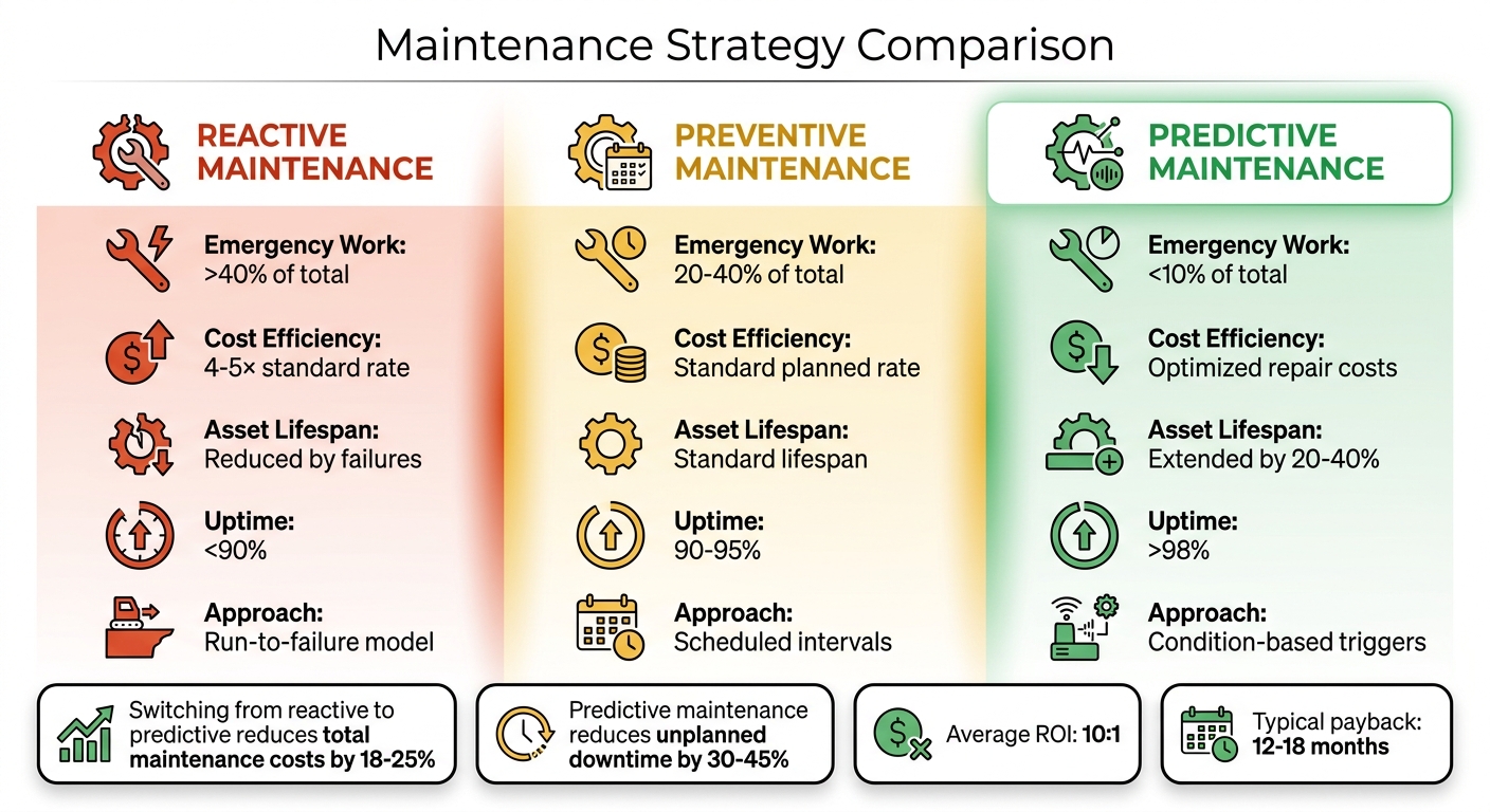
Reactive vs Preventive vs Predictive Maintenance: Cost and Performance Comparison
Bringing downtime avoidance metrics into your investment planning can turn technical savings into clear financial benefits for both capital (CAPEX) and operational (OPEX) expenditures. The key? Translate maintenance savings into financial terms your executives understand – like Net Present Value (NPV), Internal Rate of Return (IRR), and Payback Period [1].
By extending asset lifespans by 20–40% [5], you can significantly lower repair costs and delay major replacements. This frees up funds for other strategic priorities.
Focusing on asset criticality scoring ensures resources are directed where they matter most. For instance, prioritize assets where a single failure could cost more than $10,000 in downtime or trigger safety or quality issues [5]. Often, this means targeting the 20% of assets that account for 80% of maintenance costs [5]. Tools like Oxand Simeo™ help you use current maintenance data – such as spending, downtime hours, and technician counts – to project annual savings under "conservative", "moderate", or "aggressive" scenarios [1].
The "cost of doing nothing" can be a powerful motivator. For example, a VP of Operations at a multi-site industrial manufacturer found that reactive maintenance was costing $6.2 million annually due to preventable downtime, emergency overtime, and expedited parts. This justified a $420,000 Year 1 investment in a CMMS across 11 plants. Over two years (ending in 2026), they achieved a 38% reduction in unplanned downtime, saved $1.1 million in parts inventory costs, and cut overtime by 44%. By Year 2, the quantified benefit reached $4.9 million, delivering a 17:1 return on recurring costs [1].
"We didn’t lead with features – we led with the cost of doing nothing. We calculated that reactive maintenance was costing us $6.2 million per year in preventable downtime, emergency overtime, and expedited parts."
- VP of Operations, Multi-Site Industrial Manufacturer [1]
Maintaining a cost avoidance register – which logs each predictive intervention and assigns a monetary value to the failure avoided – provides clear, auditable proof of program value. This supports ongoing investment in predictive strategies.
Comparing Reactive, Preventive, and Predictive Maintenance Strategies
A deeper understanding of maintenance strategies highlights how predictive approaches align with strategic investment goals. Reactive maintenance operates on a "run-to-failure" model, where emergency work can exceed 40% of total activity and repair costs are 4–5 times higher than standard rates. Preventive maintenance, on the other hand, uses scheduled intervals to reduce emergency work to 20–40%, though it can lead to unnecessary repairs and planned downtime. Predictive maintenance relies on condition-based triggers, cutting emergency work to under 10%, optimizing repair costs, and extending asset lifespans by 20–40% [5][8][17].
Here’s a breakdown of how these strategies compare:
| Strategy | Emergency Work | Cost Efficiency | Asset Lifespan | Uptime |
|---|---|---|---|---|
| Reactive | >40% of total | 4–5× standard rate | Reduced by failures | <90% |
| Preventive | 20–40% of total | Standard planned rate | Standard lifespan | 90–95% |
| Predictive | <10% of total | Optimized repair costs | Extended by 20–40% | >98% |
Switching from reactive to predictive maintenance can cut total maintenance costs by 18–25% and reduce unplanned downtime by 30–45% [5][16]. These savings allow for smarter capital allocation and fewer emergency replacements, directly supporting long-term asset performance and financial planning.
Connecting Downtime Avoidance with Sustainability Goals
Predictive maintenance doesn’t just save money – it also supports environmental and operational goals. By ensuring equipment runs at optimal efficiency, energy consumption can drop by 15–20%, directly lowering both operational costs and the facility’s carbon footprint [5]. Extending asset lifespans by 20–40% also delays the need for new equipment, reducing resource use and the environmental impact tied to manufacturing and disposal [5].
Facilities with structured maintenance programs report 40–70% fewer safety incidents, which can lower risk-based insurance expenses and improve ESG reporting [1]. Modern investment planning increasingly includes "cost avoidance" metrics like prevented environmental fines, reduced safety incidents, and avoided compliance violations – factors often overlooked in traditional ROI models [1].
Tracking sustainability KPIs alongside downtime metrics helps demonstrate the full value of predictive maintenance. For example, energy savings can be calculated by multiplying kilowatt-hours saved by your energy rate, while extended asset life can be measured as deferred replacement costs divided by years. Together, these metrics elevate maintenance from a cost center to a strategic driver of reliability and ESG performance [18].
Conclusion
Calculating the value of avoiding downtime is a logical process. Start by pinpointing your critical assets using tools like FMEA or criticality scoring. Next, establish clear benchmarks for your current downtime hours, MTBF (Mean Time Between Failures), MTTR (Mean Time to Repair), and maintenance expenses [19][20]. Once you have these baselines, break down your downtime costs – including lost production, emergency labor, expedited parts, and overhead. From there, model potential reductions achievable through predictive maintenance, which typically delivers 35–45% less unplanned downtime and 25–30% lower maintenance costs [20].
With these baselines in place, calculating ROI becomes straightforward. Subtract the program costs from the total benefits and divide by those costs. Most manufacturers experience payback within 12–18 months [20]. The U.S. Department of Energy highlights an average 10:1 ROI for predictive maintenance programs [5]. Even a single avoided major failure can often offset the entire program investment.
Oxand Simeo™ takes ROI estimation a step further. By integrating real-time condition data with over 10,000 proprietary aging models and 30,000 maintenance laws developed over two decades, it uses probabilistic modeling to simulate asset aging, failure rates, and energy consumption. This allows users to test conservative, moderate, and aggressive scenarios to pinpoint where their investment will yield the best results – whether through deferred capital replacement, reduced emergency repairs, or asset lifespan extensions of 20–40% [5]. These advanced simulations directly align with the ROI improvements predictive maintenance offers.
Start small by piloting this approach on a handful of high-impact assets. Focus on 2–3 key assets, document the avoided failures in a cost avoidance register, and use those tangible results to support a broader implementation [19][17]. By translating maintenance savings into financial metrics like NPV (Net Present Value), IRR (Internal Rate of Return), and payback period, you can demonstrate value in terms executives understand. This shift positions maintenance not as a reactive expense but as a strategic driver of profitability and reliability. It transforms asset management into a proactive, cost-effective strategy, optimizing performance and lifecycle costs for infrastructure and real estate managers.
FAQs
What data do I need to estimate downtime costs if my records are incomplete?
To estimate downtime costs when records are incomplete, concentrate on a few essential factors. These include lost revenue during downtime, wages for idle employees, emergency repair costs, penalties for missed deadlines, and the length of the downtime period. If exact data isn’t available, rely on industry averages, past trends, or similar metrics to approximate these variables. This approach can help you piece together a more accurate understanding of downtime costs, even with limited information.
How do I choose which assets to include in a predictive maintenance pilot first?
When deciding where to begin, focus on assets that are essential to daily operations, have a track record of frequent failures, or are expensive and challenging to maintain or reach. Starting here allows for quick, noticeable gains like reducing costs and improving efficiency. Target assets where remote monitoring can make a real difference and where the return on investment (ROI) is evident. This approach creates a solid base to expand the program effectively.
How can I validate downtime-avoidance ROI without overestimating savings?
To ensure you’re not overestimating the return on investment (ROI) for downtime-avoidance strategies, stick to a structured, data-backed approach. Start by calculating the true costs of downtime. This should include production losses, labor expenses, and even those hidden costs, like emergency repairs or expedited shipping fees.
Incorporate tools like failure modeling and risk assessments. Rely on historical data and make conservative assumptions to keep your projections grounded in reality.
Measure key performance indicators (KPIs) such as downtime frequency, duration, and associated costs. By comparing data from before and after implementation, you can confirm that your savings estimates are based on actual evidence rather than guesswork.