


You do not need perfect data to build a carbon baseline. If I had to boil the article down to one point, it would be this: set the rules first, use the best data you have, label every estimate, and focus on the few assets that drive most emissions.
For large U.S. real estate and infrastructure portfolios, the biggest problems are usually the same: missing utility bills, mixed meter setups, weak asset records, and gaps in tenant data. But that should not stop the work. A baseline is still usable when I:
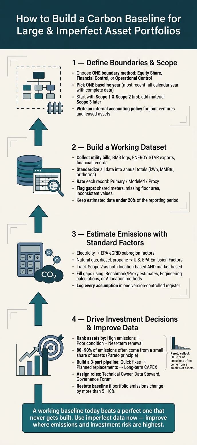
- define one boundary method and stick to it
- pick one baseline year with enough data to work from
- start with Scope 1 and Scope 2
- use direct data first, then fill gaps with estimates
- track assumptions in one place
- rank assets by emissions, condition, and renewal timing
The article also makes one point that matters for money decisions: in many portfolios, a small share of sites can drive 80%–90% of emissions. So instead of trying to clean every record at once, I would fix data at the highest-emitting assets first.
Quick Comparison
| Part of the job | What I’d do first | Why it matters |
|---|---|---|
| Boundary | Choose equity share, financial control, or control of day-to-day site activity | Keeps reporting rules the same across assets |
| Baseline year | Use the latest full year with enough records | Gives me a clean starting point |
| Scope | Start with Scope 1 and 2; add material Scope 3 later | Cuts delay and keeps the first pass focused |
| Data quality | Sort records into direct, modeled, and proxy | Makes weak spots easy to see |
| Gap filling | Use benchmark, allocation, or engineering estimates | Lets me finish the baseline even with holes |
| Decision use | Link emissions to asset condition and renewal cycles | Helps point CAPEX to the right sites |
| Updates | Review each year and restate after major portfolio changes | Keeps year-to-year results aligned |
In short, the article is not about getting every number exact on day one. It is about building a baseline that is clear, traceable, and usable now – then improving it where the carbon and cost stakes are highest.
How to Build a Carbon Baseline for Large Real Estate Portfolios
Asset Impact and the role of asset-based data in climate action
sbb-itb-5be7949
1. Define Boundaries, Baseline Year, and Material Emission Sources
Before you calculate a single ton of CO2e, make three calls first: decide what’s inside the boundary, pick the year you’ll measure against, and choose which emission sources to include at the start.
Choose Organizational and Portfolio Boundaries
The GHG Protocol gives you three boundary approaches: Equity Share, Financial Control, and Operational Control [4].
| Boundary Approach | Reporting Logic | Best For |
|---|---|---|
| Equity Share | Emissions allocated by ownership share. | Investors and REITs with many minority stakes. |
| Financial Control | 100% if you control financial reporting and risk. | Organizations where financial risk/reward is the primary driver. |
| Operational Control | 100% if you control day-to-day operations. | Owner-operators and facility managers with direct control. |
This choice matters most when you deal with joint ventures and co-owned assets. That’s where teams often get tripped up.
In leased properties, tenant-controlled spaces usually fall under Scope 3 Category 13, while landlord-controlled common areas usually sit in Scope 1 or 2 [4][5].
Pick one approach and use it across the whole portfolio. Don’t switch logic from asset to asset. It helps to write a short internal accounting policy that spells out how you handle joint ventures and leased assets. If the rules stay fuzzy, people end up arguing about ownership instead of working on emissions cuts.
You should also set a recalculation policy early. Restate the base year after material acquisitions or disposals that change portfolio emissions by about 5% [4][1].
Once those rules are in place, you can lock in the year and the source set that will anchor the baseline.
Set the Baseline Year and Scope by Materiality
Use the most recent full calendar year with reasonably complete data [4]. If site performance swings a lot, use a three-year average to smooth out odd years.
In large, uneven portfolios, start where emissions and data quality matter most. An 80/20 screen is a good first pass: in large portfolios, a small number of assets often drive 80%–90% of total emissions [1]. Find those sites first and put more effort into data collection there.
For the long tail of smaller, lower-emitting assets, lighter estimation methods can work fine, as long as you label them clearly.
With the baseline year set, the next move is to narrow the scope to the emission sources that will shape the first round of decisions.
Decide Which Scopes to Include First
Start with Scope 1 and Scope 2. They’re usually the easiest to measure and should anchor the first baseline [1][4].
For Scope 3, begin only with material, well-supported categories such as Category 13 and, when capital works drive near-term emissions, Category 1 [4]. Log every exclusion in an assumption register and add a short reason for each one.
These boundary choices shape how you pull together and screen the records in the next step.
2. Build a Working Dataset from Incomplete Asset, Meter, and Energy Records
Once your boundaries and scope are set, start building a working dataset right away. Don’t wait for spotless records. Use what you have, and mark the holes in plain sight.
Build a Clean Asset Inventory and Map It to Energy Sources
Before you tie in energy data, each in-scope asset needs a standard record. At a minimum, include the same core fields for every site: name, address, gross floor area, primary property use, and occupancy or vacancy rate [7][6].
Be specific about floor area. Note whether it covers the full building, landlord space, common areas, or vacant space. That small detail matters. Without it, site-to-site comparisons can get messy fast [6].
Once the inventory is in shape, map each asset to the energy sources it uses, such as electricity, natural gas, district steam, and other fuels, along with the meters and utility accounts tied to that site [1][6]. This is what connects each building to the records that feed the baseline.
Standardize Utility and Fuel Data into Annual Totals
Pull energy data from every source you can get your hands on: utility bills, supplier files, ENERGY STAR Portfolio Manager exports, building management system (BMS) logs, and financial records.
Billing periods almost never line up cleanly with a baseline year. So bring everything into one reporting window – usually 12 to 24 months for a baseline – and one unit of measure, such as kWh, MMBtu, or therms [7][6].
If an asset only has part-year data, like a building that opened mid-year, annualize it with linear extrapolation. Keep a lid on estimated data: no more than 20% of the reporting period, and no more than three estimated months across two reporting years [2][9].
Rate Data Quality and Document Gaps
Not all records carry the same weight. Put each one into a simple data quality tier – primary, modeled, or proxy – based on source reliability, completeness, and level of detail [1][8]. If something is estimated, say so clearly.
Also flag the weak spots now:
- Shared meters
- Missing floor area data
- Inconsistent year-over-year values
- Sites with no direct utility bills
These are the places where you’ll need estimates in the next step. Labeling them early keeps the baseline easy to audit and easier to defend. Source quality should guide where you use direct data and where you fill gaps with estimates.
The table below shows how common data sources stack up for baselining:
| Data Source | Availability | Accuracy | Processing Effort | Best Use in Baselining |
|---|---|---|---|---|
| Utility Bills | High | High | Medium | Primary source for Scopes 1 & 2; financial reconciliation [1][6] |
| Sub-metering | Low to Medium | Very High | Low | Hotspot analysis; validating equipment efficiency [1][8] |
| BMS Logs | Medium | High | High | Identifying operational waste and peak demand patterns [1][8] |
| Financial Records | Very High | Low | Low | Spend-based proxy for Scope 3 or missing utility data [1] |
| Inspections/Audits | Low | High | Medium | Verifying asset inventories and primary energy sources [6] |
One last gut check can save a lot of cleanup later: calculate energy use intensity (EUI) for each building and compare it with regional benchmarks for that property type [6]. Big swings often point to a missing bill, bad floor area input, or some other data problem hiding in plain sight. Those flagged gaps then carry forward as assumptions and proxies in the emissions calculation step.
3. Estimate Emissions Using Standard Factors and Transparent Assumptions
Take the working dataset from Section 2 and convert each energy record into annual tCO2e using one emission factor for each fuel or energy source [2]. In a large portfolio, the aim isn’t perfect precision. It’s consistent treatment across records that vary in quality. A baseline stands up better when you use the right factors, follow one gap-filling rule set, and write down every assumption.
Convert Energy to Emissions Using U.S. Emission Factors
For electricity, use EPA eGRID subregion factors that match the year of your baseline data. For natural gas, fuel oil, diesel, propane, and gasoline, use the U.S. EPA‘s Emission Factors for Greenhouse Gas Inventories or DOE published values [2].
Scope 2 electricity adds one more choice: location-based or market-based. Track both on separate lines. The location-based method reflects the physical grid. The market-based method reflects contractual instruments such as RECs or PPAs [1]. If a site has behind-the-meter solar, subtract self-generation from grid imports before you apply the eGRID factor. But don’t subtract off-site renewable purchases in the location-based calculation [2].
Fill Data Gaps with Proxy, Allocation, and Engineering Methods
Use direct data when records are complete, and save estimates for the gaps.
Benchmark-based estimation is useful when you know the floor area and property type but don’t have meter data. Use a median EUI in kWh/ft² for that building subtype and region, then estimate fuel shares with fuel-share assumptions for that asset class [2]. If you only have partial floor-area coverage, give more weight to site data as coverage goes up [2].
Apply the same annualization rule to partial-year records that you used in Section 2.
For unmetered mechanical or process equipment, use bottom-up engineering calculations. Multiply nameplate capacity (kW) by annual operating hours and a load factor to estimate kWh, then apply the matching emission factor. This method takes more work, so use it for high-emission equipment where the extra effort makes sense [1].
Keep an Assumption Register and Segment the Results
Every factor source, benchmark reference, allocation rule, exclusion, and calculation rule should live in one version-controlled assumption register. Include the effective date of each factor and a change log. That’s what helps the baseline hold up when an auditor or board member asks why two similar buildings show different emission intensities, and it lets capital planning compare sites on the same basis [1] [2].
Once the calculations are done, split the portfolio into high-emission and low-emission tiers using both total tCO2e and intensity metrics such as tCO2e/ft² [1]. A confidence profile should show what share of portfolio emissions comes from metered data versus estimates [1]. Use that profile to separate sites that need better data from sites that are ready for investment comparison.
The table below compares the three main calculation methods across the points that matter most in a large portfolio [1] [2]:
| Method | Accuracy | Data Needs | Scalability | Defensibility |
|---|---|---|---|---|
| Direct Metered Data | High | High (invoices/meters) | Low (manual effort) | High (audit-ready) |
| Benchmark/Proxy Estimates | Moderate | Low (floor area, property type) | High (automated) | Moderate (industry standard) |
| Engineering Calculations | Moderate–High | Moderate (nameplate capacity, operating hours) | Moderate | High (technical basis) |
That emissions split becomes the input for site ranking and CAPEX prioritization.
4. Use the Baseline to Drive Investment Decisions and Data Improvements
The high-emission/low-emission split from Section 3 is your starting point. But a baseline only matters if it changes where money goes. Use that split to rank assets by emissions, condition, and renewal timing using a risk-based approach.
Link Emissions to Asset Condition, Criticality, and Renewal Timing
Start with assets that sit at the intersection of high emissions, poor condition, and near-term renewal needs. In many portfolios, a small share of assets drives most emissions. A Pareto lens helps you spot those hotspots fast [1].
That’s where the baseline starts to do real work. Emissions data on its own tells you what is heavy. Add condition scores, remaining useful life, and service criticality, and you start to see what to do first [1].
An asset already lined up for renewal in the next few years has a very different case than one in a site that was renovated not long ago. When you line these pieces up, decarbonization work can move with planned renewal cycles instead of fighting for a separate budget. After you identify hotspots, test scenarios before you commit capital.
Compare Scenarios and Build a Prioritized Project Pipeline
Build a three-part pipeline: quick operational fixes, planned replacements, and long-term CAPEX [1].
- Quick operational fixes deal with issues you can address now.
- Planned replacements focus on assets nearing end of life, where lower-carbon options can be built into the renewal cycle.
- Long-term CAPEX covers deep retrofits, fuel switching, and grid-capacity upgrades that may depend on permits or local infrastructure [1].
Then pressure-test that pipeline. Run it against high carbon-price, rapid electrification, and grid-constraint scenarios to see which projects still make sense under different futures [1]. That step helps separate projects that look good on paper from ones that can hold up when conditions shift.
Set Governance for Annual Updates and Data Improvement
A baseline that isn’t updated can turn into a problem. Assign three roles: Technical Owner, Data Steward, and Governance Forum [1]. Without clear ownership, year-over-year comparisons can drift and become hard to trust.
Use the data quality scores from Section 2 to shape a focused improvement plan. Put new meters and site surveys on the highest-emitting assets first [1]. Quarterly reviews help catch oddities early and cut down on year-end reconciliation work [6].
Set a recalculation policy up front. If a data correction, methodology update, or structural event like an acquisition changes total baseline emissions by more than 5% to 10%, that should trigger a formal restatement [3].
Use these segments to match each intervention type to the quality of data behind it:
| Portfolio Segment | Baseline Profile | Typical Interventions | Data Priorities |
|---|---|---|---|
| Carbon Hotspots | High-emitting, process-intensive assets. | Electrification, fuel switching, heat integration, and process redesign. | Primary metered data; sub-metering for specific high-intensity processes. |
| Quick-Win Candidates | Assets with high EUI or operational waste. | Equipment tuning, LED retrofits, leak reduction, and control optimization. | Monthly utility bill reconciliation; occupancy/vacancy impact analysis. |
| Hard-to-Abate Assets | Assets with high heat demand or infrastructure constraints. | Deep retrofits, low-carbon fuel transition, or long-term grid-capacity upgrades. | Engineering-grade modeled data; feasibility studies on grid/fuel constraints. |
Conclusion: A Working Baseline Today Beats a Perfect One That Never Gets Built
A useful baseline doesn’t need perfect data. It needs clear boundaries, plain estimates, and a process for improving the highest-emitting assets first.
From there, the priority is simple: put your effort where emissions and investment risk are highest. Start with assets where high emissions, poor condition, and near-term renewal overlap. Keep every assumption in one register, then recalibrate when the portfolio changes in a material way. That’s what keeps the baseline tied to actual decisions instead of letting it sit in a report.
Use annual updates to move from proxies to measured data on the sites that drive the most emissions. A baseline only matters if it changes decisions.
That’s what turns a carbon baseline into a capital planning tool. The best results come from using imperfect data now to guide capital plans while closing the biggest gaps first.
FAQs
How accurate does a carbon baseline need to be at the start?
It doesn’t need to be perfect, but it must be consistent, believable, and defensible.
Use the data you have to build a reliable, auditable baseline with clear boundaries, documented methods and assumptions, and the emission sources that matter most. It’s fine to use estimates where data is missing, as long as you document them clearly and improve them over time.
What should I do if tenant or shared-meter data is missing?
Write down your estimation method so the baseline stays consistent and easy to review. Pull all available asset data into one place, then map energy flows to show where the gaps are.
For missing consumption data, estimate it by extrapolating from similar utility records and floor area data. You can also use standard benchmarks, such as the median energy intensity for the property subtype and country. Record which values were estimated, the time period covered, and the logic behind each estimate.
How often should I update or restate the baseline?
Restate your baseline under a formal recalculation policy so it stays defensible and comparable over time.
Most teams do this after major structural changes, material methodology updates, or the discovery of major errors. It also helps to set a clear governance cadence, such as an annual review or a check after major transactions.
For auditability, keep a changelog that shows what changed, when it changed, and why. That way, your baseline doesn’t drift over time, and anyone reviewing it can follow the logic.
Related Blog Posts
- Achieving Net-Zero in Real Estate Portfolios: From Targets to Investment Plans
- Overcoming Data Gaps in Carbon Metrics: Building a Reliable Baseline for Investment Decisions
- What Makes Aging Infrastructure Portfolios Harder to Decarbonise – and What to Do About It
- What a Good Decarbonisation Investment Plan Looks Like in Practice